
Press Ctrl+ and K to search
目录
java中定时方案各式各样,今天来讲述下 xxl-job 的部署与应用
概念
XXL-JOB是一个分布式任务调度平台,其核心设计目标是开发迅速、学习简单、轻量级、易扩展。现已开放源代码并接入多家公司线上产品线,开箱即用。
特点
参考网站 https://www.xuxueli.com/xxl-job/
部署
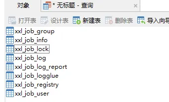
初始化数据库
请下载项目源码并解压,获取 “调度数据库初始化SQL脚本” 并执行即可。
“调度数据库初始化SQL脚本” 位置为:
sh

/xxl-job/doc/db/tables_xxl_job.sql
调度中心支持集群部署,集群情况下各节点务必连接同一个mysql实例;
如果mysql做主从,调度中心集群节点务必强制走主库;
编译源码
解压源码,按照maven格式将源码导入IDE, 使用maven进行编译即可,源码结构如下:
text

xxl-job-admin:调度中心
xxl-job-core:公共依赖
xxl-job-executor-samples:执行器Sample示例(选择合适的版本执行器,可直接使用,也可以参考其并将现有项目改造成执行器)
   :xxl-job-executor-sample-springboot:Springboot版本,通过Springboot管理执行器,推荐这种方式;
   :xxl-job-executor-sample-frameless:无框架版本;
配置部署“调度中心”
调度中心项目:xxl-job-admin
作用:统一管理任务调度平台上调度任务,负责触发调度执行,并且提供任务管理平台。
调度中心配置文件地址:
sh

/xxl-job/xxl-job-admin/src/main/resources/application.properties
调度中心配置内容说明:
properties

### web
server.port=8080
server.servlet.context-path=/xxl-job-admin

### actuator
management.server.servlet.context-path=/actuator
management.health.mail.enabled=false

### resources
spring.mvc.servlet.load-on-startup=0
spring.mvc.static-path-pattern=/static/**
spring.resources.static-locations=classpath:/static/

### freemarker
spring.freemarker.templateLoaderPath=classpath:/templates/
spring.freemarker.suffix=.ftl
spring.freemarker.charset=UTF-8
spring.freemarker.request-context-attribute=request
spring.freemarker.settings.number_format=0.##########

### mybatis
mybatis.mapper-locations=classpath:/mybatis-mapper/*Mapper.xml
#mybatis.type-aliases-package=com.xxl.job.admin.core.model

### xxl-job, datasource
spring.datasource.url=jdbc:mysql://127.0.0.1:3306/xxl_job?useUnicode=true&characterEncoding=UTF-8&autoReconnect=true&serverTimezone=Asia/Shanghai
spring.datasource.username=root
spring.datasource.password=root
spring.datasource.driver-class-name=com.mysql.cj.jdbc.Driver

### datasource-pool
spring.datasource.type=com.zaxxer.hikari.HikariDataSource
spring.datasource.hikari.minimum-idle=10
spring.datasource.hikari.maximum-pool-size=30
spring.datasource.hikari.auto-commit=true
spring.datasource.hikari.idle-timeout=30000
spring.datasource.hikari.pool-name=HikariCP
spring.datasource.hikari.max-lifetime=900000
spring.datasource.hikari.connection-timeout=10000
spring.datasource.hikari.connection-test-query=SELECT 1
spring.datasource.hikari.validation-timeout=1000

### xxl-job, email
spring.mail.host=smtp.qq.com
spring.mail.port=25
spring.mail.username=xxx@qq.com
spring.mail.from=xxx@qq.com
#授权码
spring.mail.password=xxx
spring.mail.properties.mail.smtp.auth=true
spring.mail.properties.mail.smtp.starttls.enable=true
spring.mail.properties.mail.smtp.starttls.required=true
spring.mail.properties.mail.smtp.socketFactory.class=javax.net.ssl.SSLSocketFactory

### xxl-job, access token  调度器和执行器通信用的
xxl.job.accessToken=

### xxl-job, i18n (default is zh_CN, and you can choose "zh_CN", "zh_TC" and "en")
xxl.job.i18n=zh_CN

## xxl-job, triggerpool max size
xxl.job.triggerpool.fast.max=200
xxl.job.triggerpool.slow.max=100

### xxl-job, log retention days
xxl.job.logretentiondays=30
部署项目:
nohup java -jar xxl-job-admin-2.3.0.jar &
如果已经正确进行上述配置,可将项目编译打包部署。
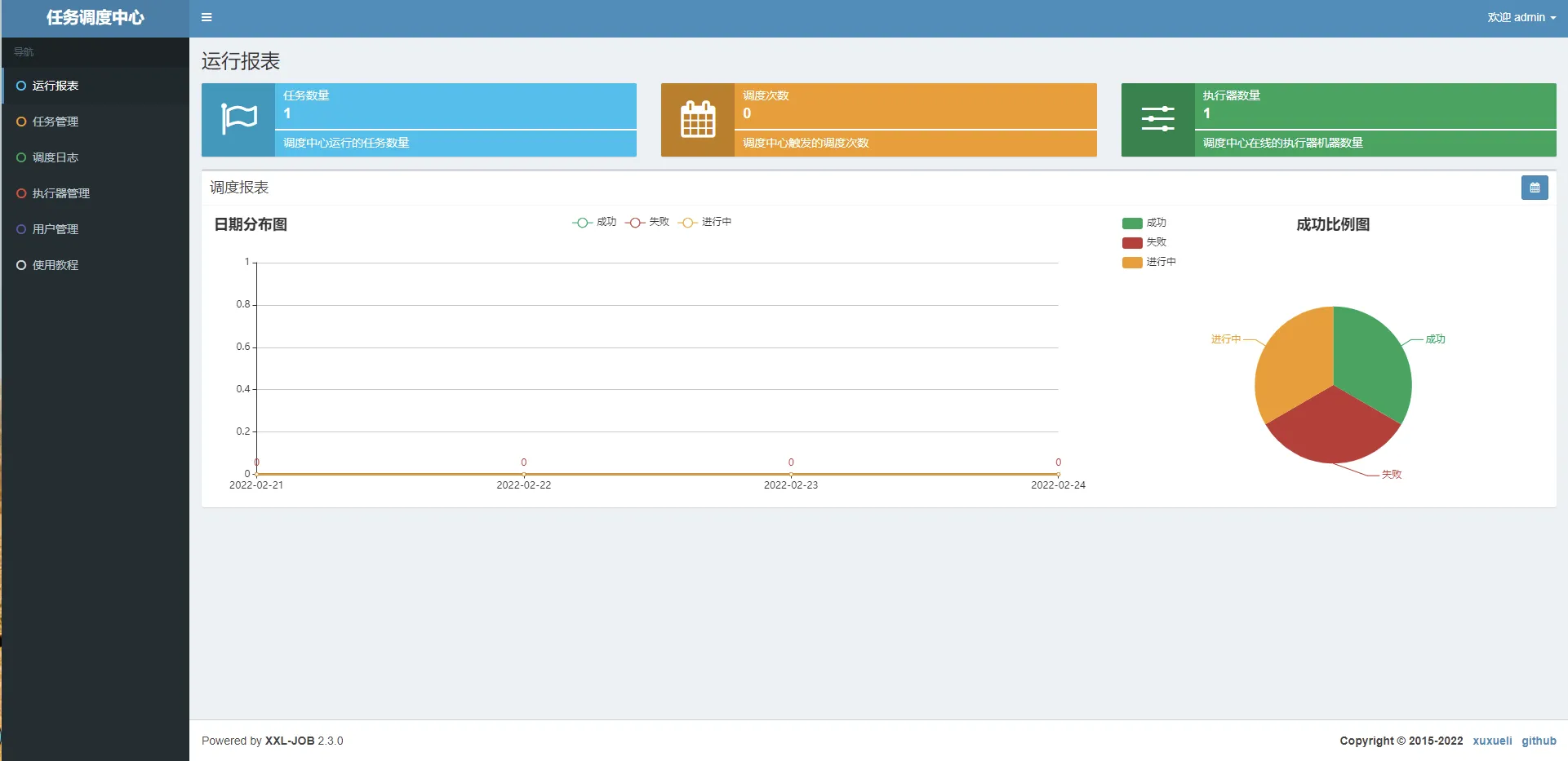
调度中心访问地址:http://localhost:8080/xxl-job-admin (该地址执行器将会使用到,作为回调地址)
默认登录账号 “admin/123456”, 登录后运行界面如下图所示。
项目整合
引入依赖
xml

 <dependency>
       <groupId>com.xuxueli</groupId>
       <artifactId>xxl-job-core</artifactId>
       <version>2.2.0</version>
   </dependency>
增加配置
xxl 属性配置文件
properties

### xxl-job executor appname
xxl.job.executor.appname=msb-item
### xxl-job executor registry-address: default use address to registry , otherwise use ip:port if address is null
###执行器注册 [选填]:优先使用该配置作为注册地址,为空时使用内嵌服务 ”IP:PORT“ 作为注册地址。从而更灵活的支持容器类型执行器动态IP和动态映射端口问题。
xxl.job.executor.address=
### xxl-job executor server-info
### 执行器IP [选填]:默认为空表示自动获取IP,多网卡时可手动设置指定IP,该IP不会绑定Host仅作为通讯实用;地址信息用于 "执行器注册" 和 "调度中心请求并触发任务";
xxl.job.executor.ip=
xxl.job.executor.port=9001
### xxl-job executor log-path
xxl.job.executor.logpath=D://logs
### xxl-job executor log-retention-days
xxl.job.executor.logretentiondays=30
客户端注入配置
java

@Configuration
public class XxlJobConfig {
   private Logger logger = LoggerFactory.getLogger(XxlJobConfig.class);

   @Value("${xxl.job.admin.addresses}")
   private String adminAddresses;

   @Value("${xxl.job.executor.appname}")
   private String appname;

   @Value("${xxl.job.executor.address}")
   private String address;

   @Value("${xxl.job.executor.ip}")
   private String ip;

   @Value("${xxl.job.executor.port}")
   private int port;

   @Value("${xxl.job.executor.logpath}")
   private String logPath;

   @Value("${xxl.job.executor.logretentiondays}")
   private int logRetentionDays;

   @Bean
   public XxlJobSpringExecutor xxlJobExecutor() {
       logger.info(">>>>>>>>>>> xxl-job config init.");
       XxlJobSpringExecutor xxlJobSpringExecutor = new XxlJobSpringExecutor();
       xxlJobSpringExecutor.setAdminAddresses(adminAddresses);
       xxlJobSpringExecutor.setAppname(appname);
       xxlJobSpringExecutor.setAddress(address);
       xxlJobSpringExecutor.setIp(ip);
       xxlJobSpringExecutor.setPort(port);
       xxlJobSpringExecutor.setLogPath(logPath);
       xxlJobSpringExecutor.setLogRetentionDays(logRetentionDays);

       return xxlJobSpringExecutor;
   }
}
修改代码
java

@Component
public class ItemScanJobHandler {
   @Autowired
   ItemScanSchedule itemScanSchedule;

   @XxlJob("itemScanJobHandler")
   public ReturnT<String> itemScanJobHandler(String param) throws Exception {
       itemScanSchedule.scanItems();
       return ReturnT.SUCCESS;
   }
}
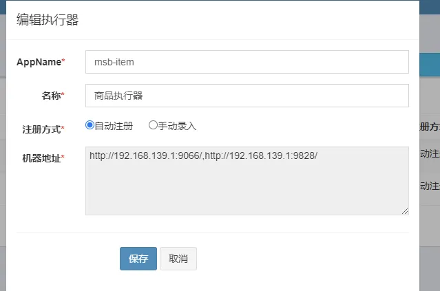
创建执行器
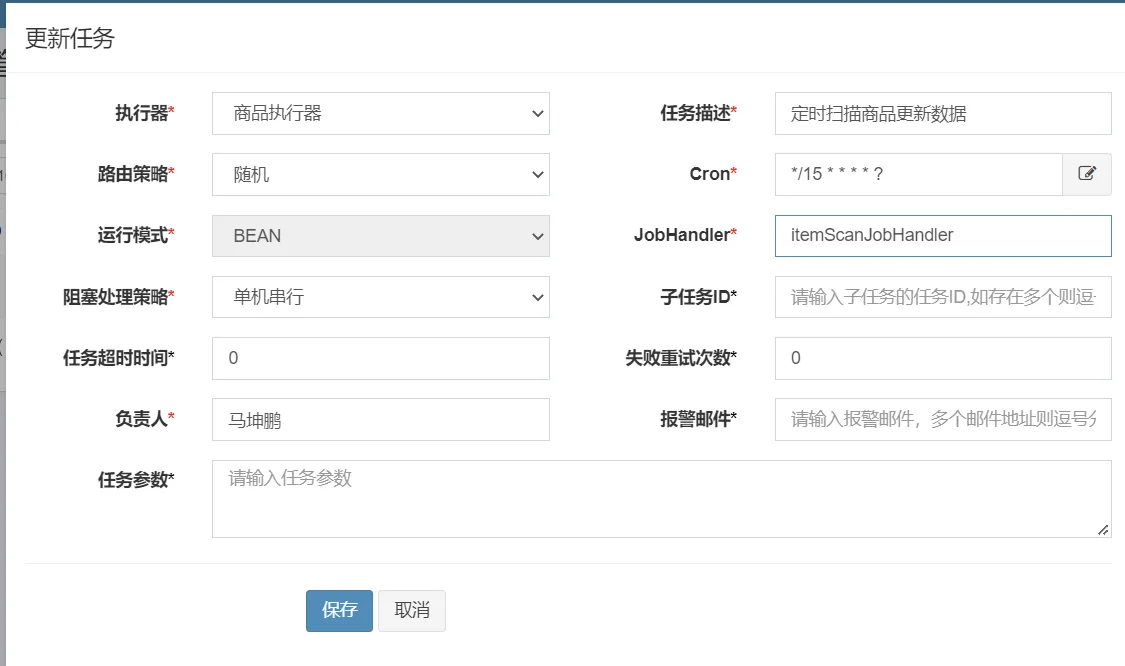
新增定时任务
本文作者:ZhangHao
本文链接:
版权声明:本博客所有文章除特别声明外,均采用 BY-NC-SA 许可协议。转载请注明出处!
目录